

Next: Estimation with unknown exposure
Up: . Introduction: Variable gain image
Previous: Robust statistics and yet
A simplified, though artificial situation, is when the camera is held
still and the exposure is adjusted manually. Although not so realistic
in today's world of mostly automatic cameras, this situation helps
provide insight into the problem.
Here, a dataset of subject matter differing only in exposure,
is used to calibrate the system. The sequence is from a dark interiour looking
out into bright sunlight, with bright sky in the background, the dynamic
range of the original subject matter being far in excess of what can
be captured in any one of the constituent pictures.
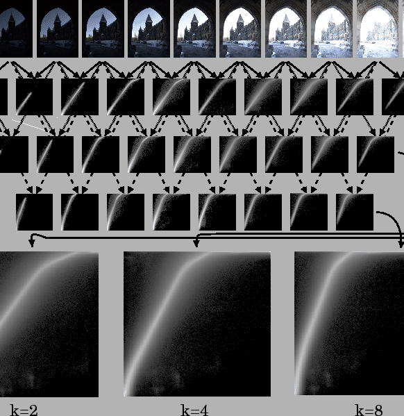
Such an image sequences is shown in Fig 3.
Figure 3:
A sequence of
differently exposed pictures of overlapping subject matter.
Such variable gain sequences give rise to a family of
comparagrams. In this sequence the gain happens to have
increased from left to right.
The square matrix  (called a comparagram)
that arose from (15) is shown for each
pair of images
under the image pairs themselves, for
  .
The next row shows pairwise comparagrams for skip=2
e.g.
  , and then for skip=3, e.g.
  .
Various skip values give rise to families of comparagrams that
capture all the necessary exposure difference information.
Each skip value provides a family of comparagrams.
 |
The comparagram (the square matrix  that arose from (15))
is a very powerful tool for understanding
the relationship between differently exposed pictures of the same subject
matter since it contains all that can be known about the response function
of the imaging apparatus [7].
Fig 3 shows the variable image sequence
together with comparagrams for various successive pairs of images
as indicated.
In this case, rather than considering all possible pairs of images
in a least squares unrolling of the comparagrams, it is only necessary
to consider the three possible pairs of comparagrams to get a total least
squares estimate.
Reverse engineering (e.g.
discovering or determining) the response function from the comparagram
may be achieved through a logarithmic unrolling of the comparagram,
as if it were a logistic map [2]. Applying a least squares
unrolling to this data provides the recovered response function shown in
Fig 4(a).
Figure:
(a) A least squares solution to the data shown in
Fig 3, using
a novel multiscale smoothing algorithm, is shown as
a solid line. The plus signs denote known ground truth data
measured from the camera using professional laboratory
instruments (as described later in this paper).
(b) The derivative of the computed response function is
the certainty function. Note that despite the excellent
fit to the known data, the certainty function magnifies
slight roughness in the curve.
 |
This solution recovers
a lookup table, for converting an image into lightspace [7].
Although this estimate of the response function,  looks reasonable, next to known points found with professional lab
equipment, we can gather more insight by plotting the derivative
(known as the certainty function [7]) of the
response curve.
This certainty function is shown in
Fig 4(b).
The resulting recovered response function,  ,
of Fig 4(a),
found by unrolling the comparagrams, can be verified
by regenerating ordered pairs
 as shown
in Fig 5.
Figure 5:
Verification of compargram unrolling:
The response function  is unrolled from the
comparagrams. A comparametric plot of the data for
each response function is made, as ordered pairs
 as a comparagram image with
bin counts equal to zero where the comparametric equation
is not true. If we compare these images with
the original comparagrams, we can easily verify that
the estimates of the response function must have been
very close to correct. Note that this method of verification
does not require any special laboratory instruments.
 |


Next: Estimation with unknown exposure
Up: . Introduction: Variable gain image
Previous: Robust statistics and yet
Steve Mann
2002-05-25


![]() that arose from (15))
is a very powerful tool for understanding
the relationship between differently exposed pictures of the same subject
matter since it contains all that can be known about the response function
of the imaging apparatus [7].
Fig 3 shows the variable image sequence
together with comparagrams for various successive pairs of images
as indicated.
that arose from (15))
is a very powerful tool for understanding
the relationship between differently exposed pictures of the same subject
matter since it contains all that can be known about the response function
of the imaging apparatus [7].
Fig 3 shows the variable image sequence
together with comparagrams for various successive pairs of images
as indicated.
![]() ,
of Fig 4(a),
found by unrolling the comparagrams, can be verified
by regenerating ordered pairs
,
of Fig 4(a),
found by unrolling the comparagrams, can be verified
by regenerating ordered pairs
![]() as shown
in Fig 5.
as shown
in Fig 5.